Current World Environment

Introduction

Particulate matter is an ambient respiratory particle suspended in the air. It has been attracting scientific attention because of its effects on human health (Shahraiyni & Sodoudi, 2016). PM₁₀ (particulate matter with size less than 10 μm) is considered to be one of major air pollutants. One of major sources of PM₁₀ is from biomass burning, brought by haze. This has becoming a typical and reoccurring challenge in Southeast Asia since 1980s (Shaadan et al., 2015). Other than that, motor vehicle usage and industrial activities also contribute to emission of PM₁₀. PM₁₀ is more hazardous to human health compared to other pollutants such as carbon monoxide and ground-level ozone (Kim et al., 2015; Ny & Lee, 2010). One study suggested that PM₁₀ increases the risk of children (between 5 to 15 years old) with asthma to visit emergency department (Cadelis et al., 2014). Also, short to medium-term exposure to PM₁₀ among infants leads to risk of respiratory syncytial virus (RSV) bronchiolitis (Carugno et al., 2018).

Located in Malaysia, Kota Kinabalu experiences monsoon season twice a year: northeast monsoon (NEM) and southwest monsoon (SWM). NEM originates from China and northern Pacific, while SWM originates from deserts in Australia. NEM occurs between November to March and is characterized by cool temperature (Ho et al., 2013). Meanwhile, SWM occurs between May to September as climate becomes warmer. According to Teong et al., (2017), SWM recorded greater amount of rainfall compared to NEM. Outside monsoon season is known as inter-monsoon, happening on April and October (Naing et al., 2011). Inter-monsoon during April is characterized by hot and dry climate, while inter-monsoon in October is cooler and has higher rainfall (Teong et al., 2017).

Short-term prediction of PM₁₀ concentration is essential as it enables community to reduce health risks by early preventive measures. Meanwhile, long-term forecasting model is crucial for urban planning, transportation networks, industrial and residential area management in such a way that minimizes health risks to public (Shahraiyni & Sodoudi, 2016). This is important for developing city such as Kota Kinabalu. Prediction model may become more accurate when seasonal factor such as monsoon is considered. This is because climate may affect PM₁₀ concentration differently, depending on season. However, it has not been studied yet whether monsoonal clustering may show difference in PM₁₀ variation with respect to meteorological and pollutant factors. Hence, this study aims to find out whether monsoonal clustering for Kota Kinabalu, Sabah shows difference with unclustered data.

Data and Methods

This research focuses on Kota Kinabalu (5.98° N, 116.07° E, altitude: 13 m), capital city of Sabah, Malaysia. As shown in Figure 1, Kota Kinabalu is located at west coast of Sabah. The climate in Kota Kinabalu is characterized by hot and humid climate, influenced by circulation of monsoons (Ho et al., 2013). Kota Kinabalu experiences uniformly high and invariant temperature and high humidity. Heavy rainfall recorded usually occurs in the afternoon (Djamila et al., 2011). In terms of economic activity, Kota Kinabalu is the gateway to the islands of Borneo. Consequently, activities such as trade, industry and tourism are concentrated in Kota Kinabalu (Noor et al., 2014).

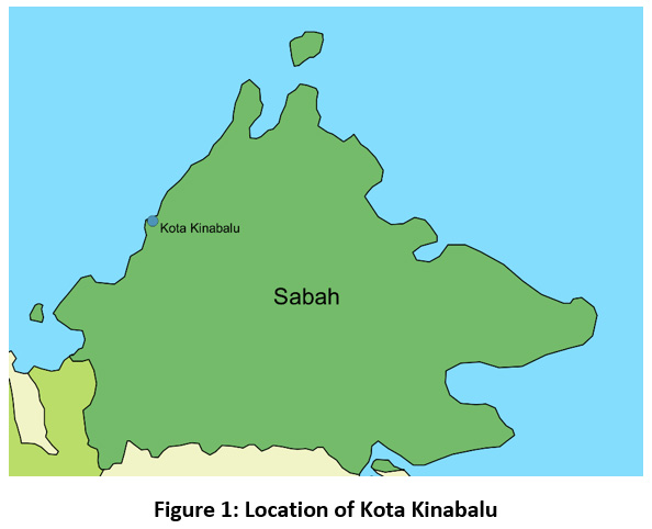Figure 1: Location of Kota Kinabalu Click here to view Figure

Air quality monitoring station, located in SMK Putatan, Kota Kinabalu is operated by Alam Sekitar Sdn. Bhd. (ASMA), a private company working under Department of Environment Malaysia (DOE). PM₁₀ concentration in μg m^-3 is measured in this station using tapered element oscillating microbalance (TOEM), with temporal resolution of 1 h. Along with other meteorological data Ws (wind speed), Wd (wind direction), Hum (relative humidity), Temp (ambient temperature) and air pollutant concentration data for CO (carbon monoxide), NO₂ (nitrogen dioxide), O₃ (ozone), SO₂ (sulfur dioxide), PM₁₀ concentration data is made available by Air Quality Division under DOE. For this research, data from 2003 to 2012 is studied. Statistics of PM₁₀ concentration data collected in CA0030 from 2003 to 2012 is summarized in Table 1.

Table 1: Summary of statistics of PM₁₀ concentration data from 2003 to 2012

As Wd is angular quantity, it is not usually used for principal component analysis or regression analysis (Gvozdic et al., 2011). Furthermore, higher magnitude of Wd does not reflect higher intensity of that property, which may present inaccuracy in both principal component analysis and regression analysis. Thus, Ws and Wd are transformed into east-west component (Wx) and north-south component (Wy) of wind speed using equations (1) and (2). Positive values indicate wind blowing eastward and northward respectively (Gvozdic et al., 2011).

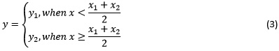
Some data from monitoring stations are missing either due to power outage, calibration, or relocation of monitoring station. Due to missingness of data, it must be imputed before it is used for this research. Data imputation is crucial for further analysis that requires complete dataset such as principal component analysis and Fourier analysis. One of the most common applicable method known as nearest neighbour method (Dominick et al., 2012; Li & Liu, 2014) is used in this paper. Given starting point of a gap (x₁ , y₁ ) and end point of the gap (x₂ , y₂), the interpolant y at corresponding time x can be calculated using equation (3) (Zakaria & Noor, 2018). As for Ws and Wd, nearest neighbour method is performed before both are transformed into Wx and Wy to reduce further data loss due to missingness.

3. Clustered and Unclustered Data

Data is clustered when data is grouped into a set with same characteristics. In contrast, data is unclustered when they are ungrouped. For this research, two sets of temporal clusters are tested and compared with unclustered data. Due to geographic location of Kota Kinabalu, this city experiences monsoonal season. Thus, monsoonal clustering is studied. In this case, data is divided into four groups: NEM (November to March), IM₄ (April), SWM (May to September), and IM₁₀ (October). Data is grouped based on the month the data is observed. The number of samples for all clusters are summarized in Table 2.

Table 2: Number of samples in unclustered and clustered data

4. Principal Component Analysis (PCA)

PCA is a method used to identify the most significant variable that contributes to variation (Dominick et al., 2012). This method is usually used to transform a set of variables to n new variables, known as principal component (PC). PCs account for more significant variation compared to observed variable X . Given that l is loading factor, principal component of i^th component is given by equation (4) (Gvozdic et al., 2011).

Explained variation is the total variation of data included in principal component. Usually, explained variation is highest in PC₁, followed by PC₂, and so on. Gvozdic et al. (2011) and Dominick et al. (2012) had demonstrated that the first two principal components PC₁ and PC₂ are used to create factor loading plot. This is because both PCs usually account at least 90% of variation of data, as evaluated in cumulative explained variation.

5. Fourier Analysis

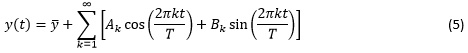
Fourier analysis involves transforming data in time domain into frequency domain using fast Fourier transform (FFT) (Kim & Son, 2011). The results obtained from Fourier analysis gives important insights on time series data (Gvozdic et al., 2011). Output from frequency domain displays cyclical behaviour of time series data as seasonal or diurnal data. Due to the nature of meteorological and air pollutant data as time series data, Fourier analysis is a suitable method in analysing the data (Gvozdic et al., 2011). A function of time series data y(t)is expressed in the form of Fourier series in equation (5), where È³ is arithmetic mean of data y(t) , T is measurement period, A_k and B_k are Fourier coefficients and k is a harmonic number.

Data transformed into frequency domain is plotted into Fourier spectrum, containing amplitudes Ck (as shown in equation (6)) as a function of frequency or period (Gvozdic et al., 2011).

Due to ability of Fourier analysis to show cyclic behaviour of time series data, this is used to verify whether variation of time series data is mainly natural or human-induced (Choi et al., 2008). It is assumed that higher amplitudes in seasonal and yearly cycle corresponds to the major effect of natural cycle while higher amplitudes in daily and weekly cycle corresponds to the major effect of anthropogenic activities (Choi et al., 2008).

Results

1. Unclustered Data

Unclustered data is analysed by inputting all data into PCA. All PCs are tabulated in Table 3, along with explained variation (EV) and cumulative explained variation (CEV). The variables with highest loading factor contribute the most in variation of corresponding principal components, and their values are highlighted in Table 3. 

Table 3: PCA of unclustered data

Note: Values smaller than 0.0001 are not shown

The explained variation is largest in first principal component and gets smaller in successive principal components. The first two principal components are considered as they take account into more than 90% of total variation of data. PC₁ and PC₂ are plotted in factor loading as shown in Figure 2. The most significant variable that contributes to variation in PC₁ is humidity, while x-component wind speed is the most significant in PC₂. This shows that 92.27% of data variation is due to both humidity and wind speed. While other variables are significant in other principal components, they are not as significant because these principal components consider only less than 10% of variation.

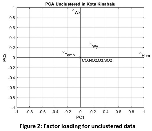Figure 2: Factor loading for unclustered data Click here to view Figure

PC₁ accounts for 83.12% of variation of dataset. At PC₁, humidity has the highest loading factor with the value of 0.9433, followed by temperature (-0.2644) and y-component wind speed (0.1668). As for PC₂ (EV = 9.15%), x-component wind speed has the highest loading factor with the value of 0.9503. Because PC₁ has significantly higher EV compared to PC₂, humidity shows to have the highest significance in variation. Meanwhile, pollutant factors (CO, NO₂, O₃, SO₂) are very close to origin of factor loading plot, which reflects insignificance in variation.

2. Clustered Data

All monsoonal clusters (NEM, IM₄, SWM, IM₁₀) are analysed using PCA, and the results are tabulated in Table 4. As cumulative explained variable for first two principal components are 92.19 ± 0.09 %, only PC₁ and PC₂ are shown in Table 4. Factor loading for all clusters are plotted as shown in Figure 3.

Table 4: Principal Component Analysis (PCA) for 4 clusters divided based on monsoonal season

Note: Values smaller than 0.0001 are not shown

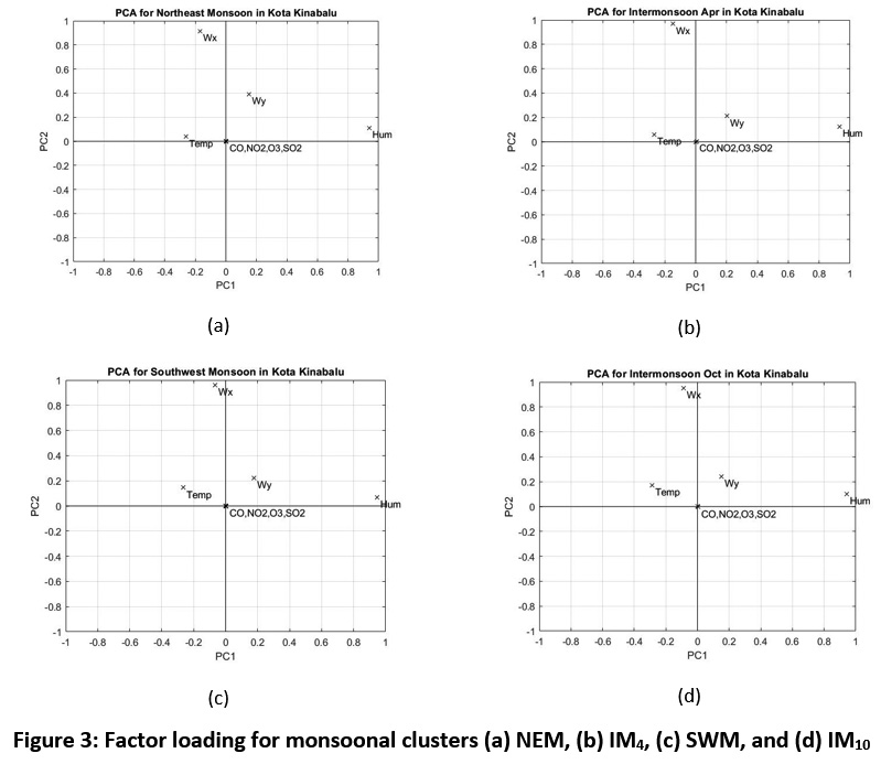Figure 3: Factor loading for monsoonal clusters (a) NEM, (b) IM4, (c) SWM, and (d) IM10  Click here to view Figure

Based on Table 3 and 4, all PC₁ and PC₂ have similar most significant variables. The values are consistent, with small discrepancies. According to EV, PC₁ accounts for 83.35 ± 1.63 % of total variation of data, with humidity having highest factor loading (0.9389 ± 0.0064), followed by ambient temperature (-0.2705 ± 0.0120) and y-component wind speed (0.1705 ± 0.0242). As for PC₂ with EV of 8.84 ± 1.58 %, x-component wind speed has shown to have highest factor loading (0.9479 ± 0.0248). Similar to unclustered data, other variables are not as significant because PC₃ and above consider less than 10% of data variation for all clusters.

3. Regression Analysis

2-D regression is plotted in Figure 4 to further analyse the variation of each parameter in response to PM₁₀ concentration for every cluster. Pollutant factors (CO, NO₂, O₃, SO₂) are not included because their variation is not significant as reflected by factor loading plot in Figure 2 and 3. According to 2-D regression in Figure 4, humidity and temperature generally show moderate to strong correlation with PM₁₀ with Pearson coefficient of correlation, ρ of -0.60 ± 0.20 and 0.63 ± 0.11 respectively. However, this is not the case for humidity in IM₄ cluster with the value of ρ = -0.37. Furthermore, humidity and temperature show strong negative correlation with each other (ρ = -0.91 ± 0.03) for all clusters.

As for wind speed, both x- and y-components generally show weak to almost no correlation towards PM₁₀ with values of ρ = 0.09 ± 0.14 and ρ = 0.24 ± 0.18 respectively. In addition, both components also exhibit weak correlation towards each other (except during SWM), humidity (except during NEM and IM₁₀) and ambient temperature.

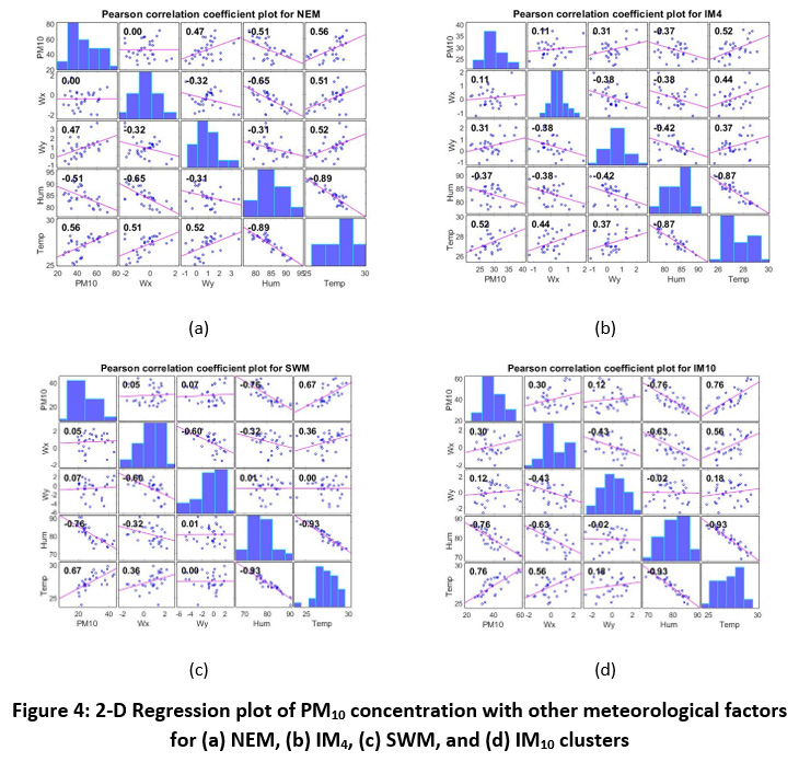Figure 4: 2-D regression plot of PM10 concentration with other meteorological factors for (a) NEM, (b) IM4, (c) SWM, and (d) IM10 clusters Click here to view Figure

4. Fourier Analysis

Fourier spectrum in Figure 5 shows three major peaks corresponding to three major cycles that affect variation of PM₁₀ concentration. Seasonal cycle is the strongest for 6-month cycle. This is attributed to monsoonal cycle. However, seasonal cycle is not as strong compared to daily and half-daily cycle. Other cycles such as weekly and monthly cycle does not show strong effect on variation of PM₁₀, as reflected by Fourier spectrum.

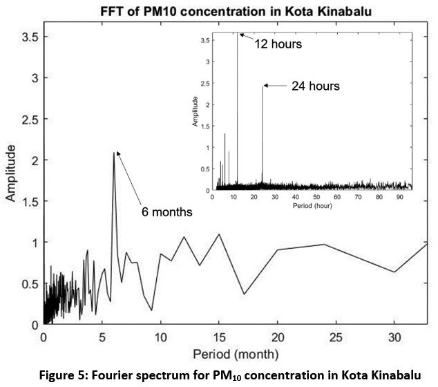Figure 5: Fourier spectrum for PM10 concentration in Kota Kinabalu Click here to view Figure

Discussion

Based on PCA and factor loading, significant variables contributing to PM₁₀ variation for monsoonal cluster does not have much difference when comparing with unclustered dataset. This is reflected by small discrepancies between factor loadings in every cluster as well as unclustered data. As clustered data shows almost similar PCA result with unclustered data, monsoonal clustering is not necessary when it comes to prediction of PM₁₀ concentration in Kota Kinabalu. This is further supported by Fourier spectrum as shown in Figure 5. Based on assumption by Choi et al., (2008), PM₁₀ concentration cycle is mainly affected by human activities. Daily activities such as traffic congestion, industries and night markets emit PM₁₀ particles (Chang et al., 2018), consequently contributing to temporal variation of PM₁₀ concentration. High amplitude of daily and half-daily cycle implies that the effect of human-induced activities is dominant over seasonal phenomenon (Choi et al., 2008).

Statistical analysis shows that PM₁₀ concentration in Kota Kinabalu decreases as humidity increases. In addition, PM₁₀ concentration shows weak negative correlation with humidity as Pearson coefficient of correlation is -0.60 ± 0.20. According to raw data, humidity in Kota Kinabalu almost always exceeds 40%. Also, monthly average humidity in Kota Kinabalu is always above 77% based on Figure 4. At high humidity level, water in air almost reaches saturation. As a result, water becomes more easily condensed and rainfall becomes easier to occur (Lou et al., 2017). This causes washout effect and wet deposition by rain on PM₁₀. At high humidity level, particulate matter absorbs water molecule and becomes heavy enough to be deposited (Munir et al., 2017). At the beginning of rainfall, small raindrop amount and dust emission from the raindrops may raise PM₁₀ concentration until certain extent (Lou et al., 2017). This may result in weak correlation between PM₁₀ concentration and humidity.

Moderate to strong correlation is also exhibited between PM₁₀ concentration and ambient temperature. This is reflected by Pearson coefficient of correlation of 0.63 ± 0.11. This may be due to atmospheric instability and enhanced kinetic motion of particles (Munir et al., 2017). High ambient temperature allows resuspension of particles into air. Furthermore, ambient temperature is strongly and negatively correlated towards humidity (ρ = -0.91 ± 0.03). The decrease in humidity inhibits deposition of particles, thus further increases PM₁₀ concentration in the air.

Both x- and y-components of wind speed are weakly correlated towards PM₁₀ concentration. This is observed by values of ρ = 0.09 ± 0.14 for eastern component and ρ = 0.24 ± 0.18 for northern component. It is possible that wind speed facilitates the dispersion of the particles (Munir et al., 2017). However, the dispersion is not fixed and can be both towards and away from Kota Kinabalu, which contributes to weak correlation between wind speed and PM₁₀ concentration.

Conclusion

In Kota Kinabalu, clustering method is not necessary when prediction of PM₁₀ concentration is made. This is because monsoonal clustering shows small difference with unclustered data. Fourier analysis further confirms this result by showing that seasonal cycle of PM₁₀ concentration is not as strong as daily and half-daily cycle. According to regression analysis, humidity and temperature both affect PM₁₀ concentration based on respective values of ρ = -0.60 ± 0.20 and ρ = 0.63 ± 0.11. This may be due to high humidity level and strong negative correlation towards each other. On the other hand, components of wind speed show weak correlation towards PM₁₀, probably due to random dispersion of particles towards and away from Kota Kinabalu.

Results from this research suggests that prediction model for PM₁₀ concentration in Kota Kinabalu does not require temporal clustering. However, future research requires study to investigate whether this applies for other parts of Sabah. Also, other types of clustering such as humidity level have yet to be studied up until now.

Acknowledgements

The authors would like to thank Universiti Malaysia Sabah for supporting this research by providing grant (SBK0324-2018, SGI0054-2018 and GUG378-2019) and Department of Environment Malaysia for providing meteorological and pollutant data for research purpose.

Funding

The authors received financial support from Universiti Malaysia Sabah via research grants (SBK0324-2018, SGI0054-2018, GUG0378-2019) for research, authorship, and publication of this article.

Conflict of Interest

The authors do not have any conflict of interest.

References

1. Cadelis, G., Tourres, R. & Molinie, J. 2014. Short-Term Effects of the Particulate Pollutants Contained in Saharan Dust on the Visits of Children to the Emergency Department due to Asthmatic Conditions in Guadeloupe (French Archipelago of the Caribbean). PLOS ONE. 9(3): 1 – 1 https://doi.org/10.1371/journal.pone.0091136
2. Carugno, M., Dentali, F., Mathieu, G., Fontanella, A., Mariani, J., Bordini, L., Milani, G. P., Consonni, D., Bonzini, M., Bollati, V. & Pesatori, A. C. 2018. PM₁₀ exposure is associated with increased hospitalizations for respiratory syncytial virus bronchiolitis among infants in Lombardy, Italy. Environmental Research. 166(2018): 452 – 457. https://doi.org/10.1016/j.envres.2018.06.016
3. Chang, H. W. J., Chee, F. P., Kong, S. K. S. & Sentian, J. 2018. Variability of the PM₁₀ concentration in the urban atmosphere of Sabah and its responses to diurnal and weekly changes of CO, NO₂, SO₂ and Ozone. Asian Journal of Atmospheric Environment. 12(2): 109 – 126. https://doi.org/10.5572/ajae.2018.12.2.109
4. Choi, Y. S., Ho, C. H., Chen, D., Noh, Y. H. & Song, C. K. 2008. Spectral analysis of weekly variation in PM₁₀ mass concentration and meteorological conditions over China. Atmospheric Environment. 42(2008): 655 – 666. https://doi.org/10.1016/j.atmosenv.
   2007.09.075
5. Djamila, H., Ming, C. C. & Kumaresan, S. 2011. Estimation of exterior vertical daylight for the humid tropic of Kota Kinabalu city in East Malaysia. Renewable energy. 36(2011): 9 – 1 https://doi.org/10.1016/j.renene.2010.06.040
6. Dominick, D., Juahir, H., Latif, M. T., Zain, S. M., & Aris, A. Z. 2012. Spatial assessment of air quality patterns in Malaysia using multivariate analysis. Atmospheric Environment, 60: 172–181. https://doi.org/10.1016/j.atmosenv.2012.0021
7. Gvozdic, V., Kovac-Andric, E. & Brana, J. 2011. Influence of meteorological factors NO₂, SO₂, CO and PM₁₀ on the concentration of O₃ in the Urban Atmosphere of Eastern Croatia. Environmental Modelling and Assessment. 16(5): 491 – 501. https://doi.org/ 10.1007/s10666-011-9256-4
8. Ho, D. J., Dayang Siti Maryam, Jafar-Sidik M. & Aung, T. 2013. Influence of weather condition on pelagic fish landings in Kota Kinabalu, Sabah, Malaysia. Journal of Tropical Biology and Conservation. 10: 11 – 21. https://doi.org/10.1007/s10666-011-9256-4
9. Kim, C. H. & Son, H. Y. 2011. Measurement and Interpretation of Time Variations of Particulate Matter Observed in the Busan Coastal Area in Korea. Asian Journal of Atmospheric Environment. 5(2): 105 – 112. https://doi.org/10.5572/ajae.2011.5.2.105
10. Kim, K. H., Kabir, E. & Kabir, S. 2015. A review on the human health impact of airborne particulate matter. Environment International. 74: 136 – 143. https://doi.org/1016/
    j.envint.2014.005
11. Li, L. & Liu, D. J. 2014. Study on an Air Quality Evaluation Model for Beijing City Under Haze-Fog Pollution Based on New Ambient Air Quality Standards. International Joutnal of Environment Research and Public Health. 11: 8909 – 8923. https://doi.org/10.3390/ijerph110908909
12. Lou, C., Liu, H., Li, Y., Peng, Y., Wang, J. & Dai, L. 2017. Relationships of relative humidity with PM_2.5 and PM₁₀ in the Yangtze River Delta, China. Environmental Monitoring Assessment. 2017: 1 – 16. https://doi.org/10.1007/s10661-017-6281-z
13. Munir, S., Mohammed, A. M. F., Habeebullah, T. M., Morsy, E. 2017. Analysing PM_2.5 and its Association with PM₁₀ and Meteorology in the Arid Climate of Makkah, Saudi Arabia. Aerosol and Air Quality Research. 17: 453 – 464. https://doi.org/10.1007/s10661-017-6281-z
14. Naing, D. K. S., Anderios, F. & Lin, Z. 2011. Geographic and Ethnic Distribution of P knowlesi infection in Sabah, Malaysia. International Journal of Collaborative Research on Internal Medicine and Public Health. 3(5): 391 – 400.
15. Noor, H. M., Nasrudin, N. & Foo, J. 2014. Determinants of Customer Satisfaction of Service Quality: City bus service in Kota Kinabalu, Malaysia. Procedia – Social and Behavioral Sciences. 153(2014): 595 – 605. https://doi.org/10.1016/j.sbspro.2014.10.092
16. Ny, M. T. & Lee, B. K. 2010. Size Distribution and Source Identification of Airborne Particulate Matter and Metallic Elements in a Typical Industrial City. Asian Journal of Atmospheric Environment. 4(1): 9 – 19. https://doi.org/10.4209/aaqr.2010.10.0090
17. Shaadan, N., Jemain, A. A., Latif, M. T. & Mohd. Deni, S. 2015. Anomaly detection and assessment of PM₁₀ functional data at several locations in the Klang Valley, Malaysia. Atmospheric Pollution Research. 6: 365 – 375. https://doi.org/10.5094/APR.2015.040
18. Shahraiyni, H. T. & Sodoudi, S. 2016. Statistical Modeling Approaches for PM₁₀ Prediction in Urban Areas; A Review of 21st-Century Studies. Atmosphere. 7: 1 – 24. https://doi.org/10.3390/atmos7020015
19. Teong, K. V., Sukarno, K., Chang, H. W. J., Chee, F. P., Ho, C. M., Dayou, J. 2017. The Monsoon Effect on Rainfall and Solar Radiation in Kota Kinabalu. Transactions on Science and Technology. 4(4): 460 – 465.
20. Zakaria, N. A. & Noor, N. M. 2018. Imputation Methods for Filling Missing Data in Urban Air Pollution Data for Malaysia. Urbanism. 9(2): 159 – 166.