Net Primary Production Geography of Forest-Forming Species in Climate-Induced Gradients of Eurasia
DOI: http://dx.doi.org/10.12944/CWE.12.3.09
When using biomass and net primary production (NPP) databases compiled by the authors for 6 forest-forming species in a number of 6694 and 2242 sample plots correspondingly, a system of regression models of their NPP is designed and some species-specific regularities of NPP distribution in two climatic gradients (natural zonality and climate continentality) are stated. It is found that according to a zonal gradient, aboveground and total NPP in 2-needled pine and spruce-fir forests are monotonically increasing in the direction from the northern to the southern tip of the continent, while larch and birch have the maximum in the southern moderate and aspen and poplar - in the northern moderate zone, but oak forests do not show any significant pattern. Within a single zonal belt the aboveground and total NPP of coniferous and deciduous are monotonically decreasing in direction from the Atlantic and Pacific coasts to the continentality pole in Yakutia. The understory NPP of all the species, except oak, monotonically increasing towards the subequatorial zone. For oak forests any clear regularity is not revealed. Within a single zonal belt, when approaching continentality pole, Pinus and Quercus NPP monotonically decreases and in others species is increasing. Species-specific patterns in changing the relative indices of NPP (forest stand underground NPP to aboveground one and forest understory NPP to total forest stand one) in gradients of the natural zonality and climate continentality are established.
Copy the following to cite this article:
Usoltsev V. A, Shobairi S. O. R, Chasovskikh V. P. Net Primary Production Geography of Forest-Forming Species in Climate-Induced Gradients of Eurasia. Curr World Environ 2017;12(3). DOI:http://dx.doi.org/10.12944/CWE.12.3.09
Copy the following to cite this URL:
Usoltsev V. A, Shobairi S. O. R, Chasovskikh V. P. Net Primary Production Geography of Forest-Forming Species in Climate-Induced Gradients of Eurasia. Curr World Environ 2017;12(3). Available from: http://www.cwejournal.org/?p=17833
Download article (pdf)
Citation Manager
Publish History
Select type of program for download
| Endnote EndNote format (Mac & Win) | |
| Reference Manager Ris format (Win only) | |
| Procite Ris format (Win only) | |
| Medlars Format | |
| RefWorks Format RefWorks format (Mac & Win) | |
| BibTex Format BibTex format (Mac & Win) |
Article Publishing History
| Received: | 2017-08-23 |
|---|---|
| Accepted: | 2017-10-17 |
Introduction
At the climate summit in Paris in 2015 December 196 countries pledged to reduce carbon emissions and prevent rising average temperatures more than 2°C by the end of the century. The important role in this relation is belonging to forest ecosystems, as sinks for atmospheric carbon. The ability of forests to withdraw the carbon from the atmosphere and produce organic matter is the basis of their functioning1. Currently, the world is actively being improved the technologies estimating the carbon-depositing function of forest cover, with the most acute shortage of empirical information on the biological productivity of forests, obtained on sample plots. Experimental data on biological productivity of forests are of paramount importance for the evaluation of their role in the global biosphere cycles.2 deals with the study of the biological productivity of ecosystems as a fundamental ecological direction and as a forerunner and a basic part of modern scientific direction, namely accounting the carbon cycle in the biosphere.
The first Russian ecologist,3 examining ways to increase the productivity of the biosphere, stressed that "it is necessary to inventory our living environment as accurately as possible" (P.12). Any researcher who is attempting to inventory forest ecosystems in any aspect, is faced firstly with extremely high complexity of their structure: the presence of multistage canopy, differentiation of foliage in his profile, chaos in crown architectonics as well as in ratio of crown wood and bark, elusive mosaic of understory. However,4 offer to researchers of biological productivity of forests to be guided by the following basic thesis: «The manifest complexity in which forests exceed other communities is not a handicap but an opportunity. It makes possible measurements within the forest community by which we can learn much about its functional design, while we also obtain more satisfactory estimates of net productivity than might otherwise be possible» (P. 58).
In 1960-s a real breakthrough in this direction was carried out as a result of the implementation of the International Biological Program (IBP), and for many plant biomes the previously absent information was first obtained. Currently, biological productivity of forests is seen as their main characteristic that determines the course of processes in forest ecosystems and is used to assess the carbon-depositing capacity of forests, environmental monitoring, sustainable forest management, forest productivity modelling, taking into account global changes, study the structure and biodiversity of forest cover5. Study of biological productivity of forest ecosystems are and will be essential until solutions are needed on the problems such as global change, sustainable development and biodiversity conservation6.
Background of Research
Net primary production (NPP) is a pure carbon sink from the atmosphere in the vegetation cover and therefore it is widely used as an indicator of the intensity of the sequestration of atmospheric CO2 into terrestrial ecosystems, i.e. of their carbon depositing ability. NPP is a rate of absorbtion of atmospheric CO2 by vegetation cover (gross primary production GPP) minus returning carbon to the atmosphere by respiration of plants. The latter is characterized by great uncertainty and very unstable estimates.7;8;9
An alternative is to estimate NPP by measurement methods on forest sample plots. The first such attempt was made by German forester Ernest Ebermayer even in the 19th century. In the forests of beech, fir and pine aged between 30 to 120 years old NPP (in some approximation) was estimated as the sum of the annual increment of trees (tree stems with branches and roots) and litterfall in absolutely dry condition. The influence of age on the value of NPP was not obvious, and it was averaged respectively as 6.5, 6.4 and 6.4 tons of dry matter per 1 ha. It was first estimated also annual carbon deposition in number, respectively, 2.98, 3.06 3.07 and t/ha.10
Aboveground NPP and annual biomass increment are concepts of equal, almost identical, since the first exceeds the second on the value of losses related to defoliation of some needles and shoots of the current year by phytofagous insects, with rainfall nutrient run-off, etc., and this difference is negligible. Therefore aboveground NPP and annual increment of aboveground biomass are essentially synonymous, since the difference between them is within the accuracy of the estimation.
«The global pattern of plant biomass and biomass production is the template that has shaped the evolution of life on Earth. Assumptions about the global pattern of productivity have also shaped many aspects of ecological and evolutionary theory, particularly those related to biodiversity, speciation, population dynamics, resilience, rarity, and conservation», - have wrote.11 Relationship between biomass and NPP has strong theoretical reasons: “biomass is a direct function of productivity, and both are limited by similar ecological factors, such as moisture availability, temperature and nutrient availability”12 although the value of biomass depends on other unrecorded factors.
Although forest NPP and biomass are defined by the same endo- and exogenous factors, but they have different nature of dependences upon these factors. Indices of biomass are rather conservative, while NPP reacts more sensitively to change of these factors, including age. For example, forest biomass and NPP decline from the certain age, but this process of NPP starts much earlier than one of biomass and it defines with the violation of balance between photosynthesis and respiration, reduced availability of the elements of soil nutrition and with decline of photosynthesis rate. i. e. it is determined by the factors to which biomass is less sensitive.13 To date, a quantitative description of the relation between NPP and biomass is extremely contradictory, and there is only the forest age from all the influencing factors.14
Forest NPP and biomass are determined by the hydrothermic regime of habitats. About the application of climatic indices when estimating the forest NPP15 stated, that no index formula does not reveal physical entity of relationships between heat, moisture and the annual wood growth, therefore the index value is not biologically caused. Use of the integrated climatic index was been justified on the early times of research the forest potential productivity, before the “computer expansion”, while the technique of multifactorial regression analysis was not yet mastered and simple single-factor relationships were only analysed. Today, when there are many standard programs the mentioned disadvantages of an integrated climatic index can be addressed by building adequate empirical models and their systems designed taking into account the differentiated by ecoregions impact of each of single climatic factors.16
17compiled dependences of NPP upon temperature and precipitation on the basis of the data of more than 1000 weather stations, evenly distributed around the globe, as well as NPP actual data obtained during the International Biological Program (Fig. 1). The same dependencies have been repeated by18 on the much more extensive global database in a number of 513 sample plots on 8 major terrestrial biomes (Fig. 2). NPP single dependencies from each of two factors are obvious (see Fig. 1), but modern NPP data in much more number plotted in dependence upon the same factors show the very different picture (see Fig. 2), where to see enough precise dependences, particularly in relation to precipitation, almost impossible. This is despite the fact that with more observations intended dependencies should be more significant.
![Fig. 1. The dependence of NPP upon annual average temperature (a) and annual precipitation sum (b) for 20 vegetation formations of the globe [17].](http://www.cwejournal.org/wp-content/uploads/2017/10/Vol12_No3_Net_Uso_Fig1-150x150.jpg) |
|
![Fig. 2. The dependence of the carbon content NPP upon annual average temperature (a) and average annual precipitation sum (b) according to 513 habitats on 8 biomes of the world [18]](http://www.cwejournal.org/wp-content/uploads/2017/10/Vol12_No3_Net_Uso_Fig2-150x150.jpg) |
|
A reason for this discrepancy, it seems, is that in the case where substantial factors defining NPP are ignored, an increase in the number of observations does not give positive results. In this case such unrecorded factors are the species composition and the main morphometric indices of forest phytocenoses, that vary in natural conditions in a wide range, overlapping the NPP variation range under the influence of the actual temperature and precipitation.
Since NPP and biomass data are several times less, than only biomass data, we use in this work both databases to obtain more reliable results. Namely, studying forest biomass geography is fulfilled according to the only biomass data, and geography of NPP fractions in dependence on biomass – is fulfilled according to the smaller only NPP database with subsequent combining of those and other results on recursive principle.19;20
Material and Methods
For this study, data of 6694 and 2192 sample plots with estimates correspondingly of biomass only and of both NPP and biomass21 were analyzed, including correspondingly: for two-needled pines (subgenus Pinus) 3020 and 920 estimations on sample plots (75% in natural stands and 25% in plantations); for Larix sp. – 540 and 116, for Picea sp. and Abies sp. - 1344 and 480, for Betula sp. - 683 and 230, for Populus sp. - 413 and 166 and for Quercus sp. - 694 and 280 estimations.
A combined analysis of different species of the same genus was possible due to the fact that different but closely related species of the genus, rather than the same species, occur throughout Eurasia (e.g. Pinus nigra in the Balkans and P. densiflora in Japan), demonstrating that the habitats of woody species are associated with specific eco-regions. The latter is known as vicariation in plant community chorology22 whereby ecologically equivalent species replace each other in the course of long-time geographical separation once they form a separate but continuous habitat. In order to explore the geographical distribution of woody NPP in the broadest geographical ranges, vicariation is inevitable to consider, and thus we included data from several vicariants in our database. Therefore, geographical analysis is made at the level of the genus involving some vicarious species. Geographical distribution of the sites contained in the database shows Fig. 3.
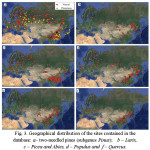 |
|
We suppose all plots were established, based on the Methodological guidelines for the International Biological Program23 in typical “background” habitats, i.e. in representative locations of plant communities. As the data were collected in many countries and under rather different ecological conditions over a longer period of time, it is assumed that the sample plots used are indeed representative and that thus they allow for an analysis of the geographic gradients of biological productivity. It is also assumed that all relevant biomass fractions were estimated following the above methodological guidelines. The relevant biomass and NPP information from the selected plots was analyzed in relation to climate related variables. We selected two quantifiable variables to describe the relevant characteristics of Eurasia: natural zonality and climate continentality.24
One way to define climatic zonality is to use the sum of effective temperatures (SET) above + 5°C or +10°C as a continuous variable. However, the known scheme of SET by25 is only established to the Northern part of Eurasia. Therefore, we used five broad climatic zones: (1) Subarctic, (2) Northern moderate, (3) Southern moderate, (4) Subtropical and (5) Subequatorial26 where the boundary between Northern moderate and Southern moderate climatic zones was defined based on the Southern boundary of Southern taiga by.27
Figure 4 shows both the geographical distribution of these zones and the geographical locations of the sample plots within the zones. The above numbers are not continuous variables, however, such serial variables (e.g., Kraft’s tree class from I to V, tree height class from I to X, site index from I to V etc.) were commonly used in modeling of forest dynamics28;29;30 as a semi-continuous proxy for modeling variables that could otherwise not be accounted for, and we treat them as such.
There are a number of formulas to quantify the degree of climatic continentality31, that mainly differ in the relative contribution and/or ratios of two components: one, the amplitude of temperatures of the warmest and the coldest months, and two, the geographical latitude. In particular, the formula by32 based on the formula by33 that we used is as follows:
K = (T - 5.4 × sinφ / T) × 100 (1)
where K is the climatic continentality index, usually varying in the range from 8 to 100; T is the amplitude of annual temperatures, °C; and φ is geographic latitude, degrees. Just like with the climatic zones, each sample plot was positioned according to the continentality index of their geographic location on the isocont map (Fig. 5).
In order to identify how climatic conditions best explain patterns of biomass and NPP, standard multivariate regression analysis is used. Assumptions and simulations obtained by regression analysis should have ecologic-geographical interpretation. NPP, as one of the characteristics of the biological productivity, is determined by climatic factors, but only as a first approximation, because there are ontogenetic, cenotic, edaphic and other levels of its variability yet. Therefore, we include into regression equations independent variables, as "explaining variability", besides climatic parameters, also stand age, tree density and growing stock. The latter is an integral index taking into account the phytocoenotic and edaphic features of forest ecosystems in a particular ecoregion.
![Fig. 4. The location of the sample plots in the climatic zones: 1 - Subarctic, 2 - Northern moderate, 3 – Southern moderate, 4 - Subtropical and 5 – Subequatorial [26; 27]. Species designations: а – subgenus Pinus; б – Larix, в – Picea and Abies, г – Betula, д – Populus and е – Quercus.](http://www.cwejournal.org/wp-content/uploads/2017/10/Vol12_No3_Net_Uso_Fig4-150x150.jpg) |
Figure 4: The location of the sample plots in the climatic zones: 1 - Subarctic, 2 - Northern moderate, 3 – Southern moderate, 4 - Subtropical and 5 – Subequatorial.26;27 Species designations: a – subgenus Pinus; b – Larix, c – Picea and Abies, d – Betula, e – Populus and f – |
![Fig. 5. Allocation of the sample plots on the isocont map of Eurasia by [32]. Numbers on the map represent specific values of the Khromov’s continentality index (X axis is longitude, Y axis is latitude in degrees). Species designations see on the Fig. 4.](http://www.cwejournal.org/wp-content/uploads/2017/10/Vol12_No3_Net_Uso_Fig5-150x150.jpg) |
|
A two-stage system of related regressions was applied, namely, by recursively fitting both the climatic information and biomass/NPP data to a system of related equations of the following general form:
stage 1
N= f (A, Zon, CI)→M=f (A, N, Zon, CI)→Pi=f (A, N, V, Zon, CI) (2)
and stage 2
Zi = f (A, N, Pi, Zon, CI), (3)
where N = tree density, 1000/hа;
Ð = stand age, yrs;
V = growing stock, m3/hа;
Pi = biomass of i–th component (stems, PS; branches, PB; foliage, PF; roots, PR; aboveground biomass, PA; total biomass, PT; and understory, PU), t/hа;
Zon = the serial number of climatic zones (Fig. 4);
CI = climate continentality index (Fig. 5);
Zi = annual NPP of i–th component: stem, ZS; branches, ZB; foliage, ZF; roots, ZR; aboveground biomass, ZA; total biomass, ZT; and understory, ZU, t/hа.
Fitting equation (2 and 3) was done in the following sequence: first, N was calculated from the values of A, Zon and CI; second, V was calculated using the values of N obtained in the first stage and the same values of A, Zon and CI; third, Pi was calculated using the calculated values of N and V and the same values of A, Zon and CI; finally, Zi was calculated using the values of N, V and Pi obtained and the same values of A, Zon and CI.
When fitting the above equations, standard regression statistics were calculated. The procedure for correcting bias in logarithmic regression estimates suggested by27 was used. Note however that, due to the nature of the recursive system, the adjusted R2 values reported always refer to one step of the entire procedure, i.e. to fitting an equation to values of its variables that are taken as independent ones in that step.
Results and Discussion
The regression analysis of the system of equations (2) produced the required regression coefficients and the adjusted coefficients of determination, adjR2 (Tables 1-7). Regression coefficients of the independent variables are significant at the 95% probability level. Tabulating the equations shown in the Tables 1 and 2 is performed in the same sequence by substitution of relevant independent variables. As a result, age trends of NPP for each zonal belt are obtained and within particular belt – the same for climate continentality indices ranging from 35 to 95%.
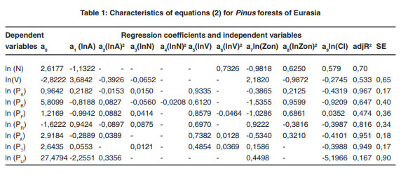 |
Table 1: Characteristics of equations (2) for Pinus forests of Eurasia click here to view table |
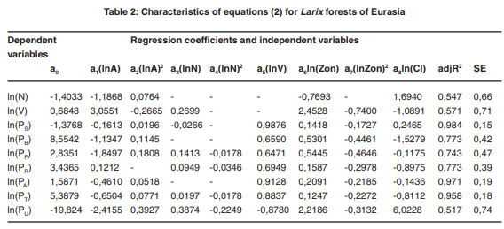 |
Table 2: Characteristics of equations (2) for Larix forests of Eurasia click here to view table |
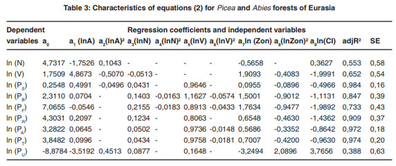 |
Table 3: Characteristics of equations (2) for Picea and Abies forests of Eurasia click here to view table |
Table 4: Characteristics of equations (2) for Betula forests of Eurasia
|
Dependent variables |
Regression coefficients and independent variables |
||||||||
|
а0 |
а1 (lnA) |
a2 (lnA)2 |
a3 (lnV) |
а4 ln(Zon) |
а5 (lnZon)2 |
а6 (lnCI) |
adjR2 |
SE |
|
|
ln(V) |
1,6658 |
1,9763 |
–0,1567 |
- |
2,5994 |
–1,4548 |
–0,6363 |
0,612 |
0,46 |
|
ln(Ps) |
–0,9678 |
0,2356 |
–0,0342 |
0,9855 |
- |
- |
- |
0,980 |
0,14 |
|
ln(Pb) |
–1,5597 |
0,2536 |
- |
0,6321 |
- |
- |
- |
0,800 |
0,34 |
|
ln(Pf) |
–5,5669 |
–0,1350 |
- |
0,4342 |
- |
- |
1,1758 |
0,475 |
0,35 |
|
ln(Pr) |
–7,3790 |
0,9400 |
–0,1271 |
0,6859 |
0,4507 |
- |
1,1510 |
0,818 |
0,31 |
|
ln(Pa) |
–0,0136 |
- |
- |
0,9132 |
- |
- |
- |
0,975 |
0,14 |
|
ln(Pt) |
0,8837 |
0,0823 |
- |
0,7313 |
- |
- |
- |
0,906 |
0,17 |
|
ln(Pu) |
–2,0045 |
0,3683 |
- |
0,2157 |
0,7952 |
- |
- |
0,319 |
0,55 |
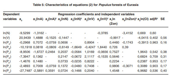 |
Table 5: Characteristics of equations (2) for Populus forests of Eurasia click here to view figure |
Table 6: Characteristics of equations (2) for Quercus forests of Eurasia
|
Dependent variables |
Regression coefficients and independent variables |
|||||||||
|
а0 |
а1(lnA) |
a2(lnA)2 |
а3(lnN) |
а5(lnV) |
a6ln (Zon) |
a7(lnZon)2 |
a8ln(CI) |
adjR2 |
SE |
|
|
ln(N) |
7,5381 |
-3,1362 |
0,2347 |
- |
- |
-2,0054 |
1,1114 |
0,5047 |
0,663 |
0,63 |
|
ln(V) |
15,1939 |
0,9191 |
- |
0,0130 |
- |
-1,3471 |
0,2027 |
-2,8197 |
0,604 |
0,48 |
|
ln(PS) |
0,2798 |
0,0457 |
- |
0,0387 |
0,9835 |
1,0585 |
-0,4329 |
-0,3530 |
0,971 |
0,15 |
|
ln(PB) |
-0,4868 |
1,5991 |
-0,1346 |
-0,0761 |
0,3251 |
0,4776 |
- |
-0,6299 |
0,727 |
0,37 |
|
ln(PF) |
-6,3228 |
0,5289 |
- |
0,0875 |
-0,0804 |
0,8818 |
- |
1,1603 |
0,352 |
0,34 |
|
ln(PR) |
-2,1096 |
0,4277 |
- |
0,2984 |
0,5461 |
0,4886 |
- |
0,0918 |
0,704 |
0,33 |
|
ln(PA) |
1,4357 |
0,5152 |
-0,0470 |
0,0155 |
0,7998 |
0,9950 |
-0,3674 |
-0,5959 |
0,951 |
0,17 |
|
ln(PT) |
3,7324 |
0,5532 |
-0,0460 |
0,0973 |
0,6994 |
0,1655 |
- |
-0,8928 |
0,932 |
0,16 |
|
ln(PU) |
20,9651 |
0,3398 |
- |
0,1917 |
0,2175 |
-8,1656 |
3,6061 |
-3,9259 |
0,247 |
0,64 |
Table 7: Characteristics of equations (3) for forest-forming species of Eurasia
|
Dependent variables and adequacy indices |
Regression coefficients and independent variables |
||||||
|
ln (ZS) |
ln (ZB) |
ln (ZF) |
ln (ZR) |
ln (ZA) |
ln (ZT) |
ln (ZU) |
|
|
Subgenus Pinus |
|||||||
|
а0 |
4,6110 |
7,9439 |
4,3347 |
-0,1120 |
4,6153 |
-0,3636 |
-12,0163 |
|
а1 (lnA) |
-0,9516 |
-0,7609 |
-0,2005 |
-1,0229 |
-0,7280 |
-0,6681 |
-0,1605 |
|
а2(lnN) |
- |
0,1070 |
-0,0623 |
0,0632 |
0,0254 |
0,1022 |
-0,0671 |
|
а3(lnPS) |
0,7770 |
- |
- |
- |
- |
- |
- |
|
а4(lnPB) |
- |
0,9659 |
- |
- |
- |
- |
- |
|
а5(lnPF) |
- |
- |
0,9364 |
- |
- |
- |
- |
|
а6(lnPR) |
- |
- |
- |
1,0591 |
- |
- |
- |
|
а7(lnPA) |
- |
- |
- |
- |
0,7564 |
- |
- |
|
а8(lnPT) |
- |
- |
- |
- |
- |
0,8453 |
- |
|
а9(lnPU) |
- |
- |
- |
- |
- |
- |
0,8905 |
|
а10(lnZon) |
0,8863 |
1,3824 |
0,4893 |
1,9949 |
0,4925 |
1,3073 |
-0,6566 |
|
a11(lnZon)2 |
-0,2197 |
-0,9099 |
- |
-0,9282 |
- |
- |
0,5901 |
|
a12(lnCI) |
-0,8841 |
-1,7834 |
-1,1184 |
- |
-0,8962 |
-0,3757 |
2,6349 |
|
adjR2 |
0,748 |
0,735 |
0,774 |
0,737 |
0,805 |
0,822 |
0,778 |
|
SE |
0,38 |
0,43 |
0,31 |
0,48 |
0,28 |
0,29 |
0,47 |
|
Genus Larix |
|||||||
|
а0 |
1,1528 |
11,9344 |
-0,8517 |
0,5231 |
1,3217 |
14,4748 |
-2,2412 |
|
а1 (lnA) |
-0,7459 |
-0,7757 |
0,5912 |
-0,6502 |
-0,5322 |
-0,4353 |
3,5265 |
|
a2 (lnA)2 |
- |
- |
-0,0789 |
- |
- |
- |
-0,3495 |
|
a3(lnN) |
- |
- |
-0,0029 |
- |
0,0392 |
0,0221 |
0,1838 |
|
a4(lnPS) |
0,6531 |
- |
- |
- |
- |
- |
- |
|
a5(lnPB) |
- |
0,8442 |
- |
- |
- |
- |
- |
|
a6(lnPF) |
- |
- |
0,9504 |
- |
- |
- |
- |
|
a7(lnPR) |
- |
- |
- |
0,4129 |
- |
- |
- |
|
a8(lnPA) |
- |
- |
- |
- |
0,8958 |
- |
- |
|
a9(lnPT) |
- |
- |
- |
- |
- |
0,7771 |
- |
|
a10(lnPU) |
- |
- |
- |
- |
- |
- |
0,4611 |
|
а11(lnZon) |
-0,1409 |
-0,4713 |
0,7798 |
-0,2767 |
0,0672 |
1,5264 |
0,2326 |
|
a12(lnZon)2 |
- |
- |
-0,3761 |
- |
-0,0896 |
-1,0019 |
- |
|
a13(lnCI) |
0,0201 |
-2,4360 |
-0,1192 |
0,3264 |
-0,2775 |
-3,2792 |
-1,5370 |
|
adjR2 |
0,693 |
0,714 |
0,960 |
0,727 |
0,847 |
0,876 |
0,869 |
|
SE |
0,50 |
0,56 |
0,16 |
0,39 |
0,30 |
0,23 |
0,29 |
|
Genus Picea and Abies |
|||||||
|
а0 |
-7,1061 |
21,9617 |
-5,9461 |
9,2816 |
-1,9458 |
-0,2236 |
2,7399 |
|
а1 (lnA) |
-0,9523 |
-0,7691 |
-0,3326 |
-0,7521 |
-0,7822 |
-0,7910 |
-0,1139 |
|
a2(lnPS) |
0,9460 |
- |
- |
- |
- |
- |
- |
|
a3(lnPB) |
- |
0,9146 |
- |
- |
- |
- |
- |
|
a4(lnPF) |
- |
- |
0,8047 |
- |
- |
- |
- |
|
a5(lnPR) |
- |
- |
- |
0,8027 |
- |
- |
- |
|
a6(lnPA) |
- |
- |
- |
- |
0,8801 |
- |
- |
|
a7(lnPT) |
- |
- |
- |
- |
- |
0,8826 |
- |
|
a8(lnPU) |
- |
- |
- |
- |
- |
- |
0,8118 |
|
a9(lnZon) |
0,6653 |
0,9967 |
0,2945 |
-0,9359 |
0,3522 |
-0,1654 |
0,9217 |
|
a10(lnZon)2 |
-0,2368 |
-0,5632 |
- |
0,2753 |
-0,2066 |
- |
-0,1412 |
|
a11(lnCI) |
1,6876 |
-4,9532 |
1,3827 |
-1,8181 |
0,6215 |
0,3020 |
-0,8983 |
|
adjR2 |
0,912 |
0,805 |
0,824 |
0,801 |
0,905 |
0,894 |
0,794 |
|
SE |
0,32 |
0,38 |
0,27 |
0,31 |
0,21 |
0,23 |
0,36 |
|
Genus Betula |
|||||||
|
а0 |
0,1543 |
9,7022 |
0,0536 |
-3,5946 |
0,3444 |
-0,2838 |
-4,7987 |
|
а1 (lnA) |
-0,8322 |
-0,8461 |
-0,0437 |
-0,7636 |
-0,5656 |
-0,5114 |
-2,2911 |
|
а2(lnA)2 |
- |
- |
- |
- |
- |
- |
0,2918 |
|
а3(lnPS) |
0,9039 |
- |
- |
- |
- |
- |
- |
|
а4(lnPB) |
- |
0,9197 |
- |
- |
- |
- |
- |
|
а5(lnPF) |
- |
- |
0,9545 |
- |
- |
- |
- |
|
а6(lnPR) |
- |
- |
- |
0,9528 |
- |
- |
- |
|
а7(lnPA) |
- |
- |
- |
- |
0,8169 |
- |
- |
|
а8(lnPT) |
- |
- |
- |
- |
- |
0,9578 |
- |
|
а9(lnPU) |
- |
- |
- |
- |
- |
- |
0,8860 |
|
а10(lnZon) |
0,4058 |
1,8186 |
0,1089 |
0,2231 |
0,2632 |
- |
1,4053 |
|
a11(lnZon)2 |
- |
-1,0139 |
- |
- |
- |
- |
-0,4818 |
|
a12(lnCI) |
- |
-2,1876 |
- |
0,7810 |
- |
- |
1,6875 |
|
adjR2 |
0,933 |
0,831 |
0,939 |
0,930 |
0,873 |
0,901 |
0,887 |
|
SE |
0,20 |
0,30 |
0,17 |
0,15 |
0,23 |
0,15 |
0,29 |
|
Genus Populus |
|||||||
|
а0 |
-4,9946 |
9,9782 |
-2,0632 |
0,6816 |
-5,0481 |
-3,9453 |
-0,9543 |
|
а1 (lnA) |
-0,8398 |
-0,8882 |
-0,0334 |
-0,8539 |
-0,5458 |
-0,4958 |
0,0926 |
|
a2(lnPS) |
1,0285 |
- |
- |
- |
- |
- |
- |
|
a3(lnPB) |
- |
1,0413 |
- |
- |
- |
- |
- |
|
a4(lnPF) |
- |
- |
0,9833 |
- |
- |
- |
- |
|
a5(lnPR) |
- |
- |
- |
0,9936 |
- |
- |
- |
|
a6(lnPA) |
- |
- |
- |
- |
0,9826 |
- |
- |
|
a7(lnPT) |
- |
- |
- |
- |
- |
1,0627 |
- |
|
a8(lnPU) |
- |
- |
- |
- |
- |
- |
0,8240 |
|
a9(lnZon) |
0,5048 |
0,9565 |
0,2757 |
-0,5199 |
-0,4759 |
0,1462 |
-0,2112 |
|
a10(lnZon)2 |
-0,1007 |
-0,5738 |
-0,1291 |
0,2107 |
0,2892 |
-0,0400 |
0,0998 |
|
a11(lnCI) |
1,0512 |
-2,2020 |
0,4588 |
- |
1,1300 |
0,6708 |
- |
|
adjR2 |
0,936 |
0,808 |
0,987 |
0,980 |
0,934 |
0,932 |
0,953 |
|
SE |
0,19 |
0,27 |
0,084 |
0,084 |
0,17 |
0,12 |
0,11 |
|
Genus Quercus |
|||||||
|
а0 |
-0,9491 |
7,8360 |
-1,1425 |
0,9308 |
-4,5682 |
-5,3234 |
-12,8651 |
|
а1 (lnA) |
-1,8305 |
-0,8997 |
-0,0533 |
-0,8823 |
1,1708 |
1,3821 |
-0,0363 |
|
а2(lnA)2 |
0,1211 |
- |
- |
- |
-0,1852 |
-0,2231 |
- |
|
а3(lnPS) |
0,9279 |
- |
- |
- |
- |
- |
- |
|
а4(lnPB) |
- |
1,0796 |
- |
- |
- |
- |
- |
|
а5(lnPF) |
- |
- |
1,0620 |
- |
- |
- |
- |
|
а6(lnPR) |
- |
- |
- |
1,0427 |
- |
- |
- |
|
а7(lnPA) |
- |
- |
- |
- |
0,5614 |
- |
- |
|
а8(lnPT) |
- |
- |
- |
- |
- |
0,6820 |
- |
|
а9(lnPU) |
- |
- |
- |
- |
- |
- |
0,7707 |
|
а10(lnZon) |
-1,0834 |
0,7106 |
1,2460 |
-1,1491 |
1,0945 |
1,5734 |
2,5905 |
|
a11(lnZon)2 |
0,5898 |
-0,4719 |
-0,7403 |
0,5252 |
-0,3949 |
-0,6510 |
-1,2610 |
|
a12(lnCI) |
0,8648 |
-1,7196 |
0,1698 |
-0,0187 |
0,4071 |
0,3528 |
2,4659 |
|
adjR2 |
0,941 |
0,735 |
0,830 |
0,938 |
0,598 |
0,667 |
0,843 |
|
SE |
0,13 |
0,33 |
0,20 |
0,14 |
0,21 |
0,18 |
0,18 |
Change of forest NPP according to transcontinental zonal gradient
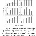
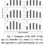
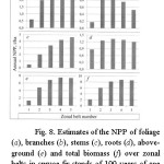
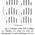
From age trends of NPP components their values are taken at the age of 50 years for the small-leaved Betula and Populus and 100 years for all other species and their dependences on zonal belt number when continentality index is equal 75-80% are built (Fig. 6-11). Analysis of the Figs. 6-11 suggests that the aboveground and total NPP of pine forests are monotonically increasing in direction from the Northern to the Southern tip of the Eurasian continent, and the same of spruce-fir forests grows with exit to the plateau in subtropical and subequatorial zonal belts. In larch and birch forests above ground and total NPP in the same gradient changes according to the bell-shaped trend with a maximum on the southern moderate zonal belt. Aboveground NPP in Populus and Quercus forests is dropping in direction from the northern moderate to the subequatorial zonal belt. Meanwhile, in the subarctic zonal belt there is no empirical data of NPP for Populus, and they cannot be for Quercus because its area in those latitudes does not apply.
 |
|
 |
|
 |
|
 |
|
Change the understory NPP according to transcontinental climatically determined gradients.
Similarly, the transcontinental trends of understory NPP of forest-forming species in Eurasia (Fig. 10) are built. NPP estimates of the understory of the forests investigated are increasing from North to South (from the subarctic to subequatorial zonal belt). They also grow in the direction from the Atlantic and Pacific coasts to the continentality pole in Yakutia, except the pine and oak forests.
![Fig. 10. Estimates of the understory NPP in pine (I), larch (II), spruce-fir (III), birch (IV), aspen-poplar (V) and oak (VI) over zonal belts when continentality index equals 80 (a), and over the [32] continen-tality indices in the southern moderate zonal belt (b). Age of birch and aspen with poplars equals 50 and of the other species 100 years.](http://www.cwejournal.org/wp-content/uploads/2017/10/Vol12_No3_Net_Uso_Fig10-150x150.jpg) |
|
![Fig. 11. Estimates of the ratio ZR/ZA in pine (I), larch (II), spruce-fir (III), birch (IV), aspen-poplar (V) and oak (VI) over zonal belts when continentality index equals 80 (a), and over the [32] continentality indices in the southern moderate zonal belt (b). Age of birch and aspen with poplars equals 50 and of the other species 100 years.](http://www.cwejournal.org/wp-content/uploads/2017/10/Vol12_No3_Net_Uso_Fig11-150x150.jpg) |
|
Change the ratio of belowground to aboveground NPP according to transcontinental climate related gradients.
The ratio of belowground to aboveground NPP (ZR/ZA) is an important characteristic of forest sustainability (root: shoot ratio) in different environmental conditions. Study on ZR/ZA values of European forests shows a variation in the range of 0.15 to 0.33, while herbaceous plants have this ratio ranged from 0.15 to 5.50, and herbaceous species have, on average, this range significantly higher than for forest ones [34].
In our study the comparison of transcontinental relative trends characterizing the ratio of belowground to overground NPP (ZR/ZA), shows a lack of patterns common to all tree species (Fig. 11). The ratio ZR/ZA in pine forests in the direction from the subarctic to subequatorial zonal belt changes according to the bell-shaped curve with a maximum at the northern moderate and southern moderate zones (Fig. 11 a), but in the direction from the Atlantic and Pacific coasts to continentality pole it increases monotonically (Fig. 11 b). The ratio ZR/ZA in birch, aspen and poplar forests increases in the direction both from the subarctic to the subequatorial zone and towards the climate continentality pole, i.e. changes opposite to that observed in the larch and spruce-fir forests.
Change the ratio of understory NPP to total one according to transcontinental climate related gradients
The ratio of understory NPP to total (above and belowground) one characterizes the relationship of two stories (upper and under), competing for living space and mutually reinforcing each other in a forest community, the ratio of which varies in different ecological and cenotic conditions. Ignoring the contribution of the understory in the carbon cycle of forest ecosystem significantly underestimates its carbon depositing ability. For example, in 60-year-old forest of Chinese pine (Pinus tabulaeformis Carr.) in Shaanxi Province, the contribution of the understory into net carbon sink makes up 37% of the total sink of the forest ecosystem [35; 36].
The results obtained suggest that both according to both ZR/ZA (see Fig. 11), and ZU/ZT (Fig. 12), no patterns common to all species. The ratio ZU/ZT in pine, larch, spruce-fir and oak forests varies according to a specific surface: in the direction of subarctic to subequatorial zonal belt there is a "failure" in the northern and southern moderate zones (with the exception of Betula and Populus), and as the climate continentality index grows, the ratio increases monotonically in all the species except pine and oak forests.
![Fig. 12. Estimates of the ratio ZU/ZT in pine (I), larch (II), spruce-fir (III), birch (IV), aspen-poplar (V) and oak (VI) over zonal belts when continentality index equals 80 (a), and over the [32] continentality indices in the southern moderate zonal belt (b). Age of birch and aspen with poplars equals 50 and of the other species 100 years.](http://www.cwejournal.org/wp-content/uploads/2017/10/Vol12_No3_Net_Uso_Fig12-150x150.jpg) |
|
Conclusions
It is found that according to a zonal gradient, aboveground and total NPP in pine and spruce-fir forests is monotonically increasing in the direction from the northern to the southern tip of the continent, while larch and birch have the maximum in the southern moderate and aspen and poplar - in the northern moderate zone, and oak forests any significant pattern do not show. Within a single zonal belt the aboveground and total NPP of coniferous and deciduous is monotonically decreasing in direction from the Atlantic and Pacific coasts to the continentality pole in Yakutia.
The understory NPP of all the species, except oak, monotonically increasing towards the subequatorial zone. For oak forests any clear regularity is not revealed. Within a single zonal belt, when approaching continentality pole, Pinus and Quercus NPP monotonically decreases and in others species is increasing.
The ratio ZR/ZA of pine forests is at maximum in the temperate zone of the latitudinal gradient, falling in both northern and southern directions, the same of larch and spruce-fir is decreases and of the other species is increases in the direction to the south. Within a single zonal belt the ratio ZR/ZA of larch, spruce-fir and oak forests is monotonically decreasing when approaching the continentality pole, while of the other species is increasing. To explain the reasons for such discrepancies is not yet possible.
The ratio ZU/ZT of pine, larch and spruce-fir forests is at maximum in the northern temperate zone of the latitudinal gradient, falling in both northern and southern directions, the same of oak forests is at minimum in the southern temperate and subtropical zonal belts and the same of the small-leaved species is monotonically raising in the southern direction. Within a single zonal belt the ratio ZU/ZT of pine forests is monotonically decreasing in the direction to the continentality pole, the same of oak forests has maximum value at continentality index equal 75 and the same of the other species is increasing.
Thus, the patterns of change of forest biomass and NPP are species-specific in two transcontinental climate induced gradients, reasons which may be multiple, and they need to be further studied. The regularities reported here are firstly obtained and have a preliminary nature: as filling the biomass and NPP database, using more sophisticated computational algorithms and due to climate change, they may be subject to offsets.
Acknowledgment
We thank the anonymous referees for their useful suggestions. This paper is fulfilled according to the programs of current scientific research of the Ural Forest Engineering University and Botanical Garden of the Ural Branch of Russian Academy of Sciences.
References
- Dylis, N.V. Fundamentals of biogeocoenology. Moscow University Publishing, 152 pp, (1978).
- Utkin, Ð.I. Study of carbon pools and fluxes at the levels of ecosystems and territorial complex, Stationary forest-ecological researches: methods, results, and prospects. Proceed. of the Conference. Syktyvkar, pp 9-12, (2003).
- Timofeev-Ressovsky, N. V. Biosphere and mankind. Scientific papers in Obninsk branch of the Geographer society of USSD, 1 (1): 3-12, (1968).
- Whittaker, R. H., Marks, P. L. Methods of assessing terrestrial productivity. Lieth H., Whittaker R.H. (eds.). Primary productivity of the biosphere. Berlin, Heidelberg, New York: Springer-Verlag, P. 55-118, (1975).
- Fowler, A., Low, K., Stone, J. Earth observation for sustainable development: Using space-based technology for monitoring Canada’s forests. Information Forestry, Canadian Forest Service, Pacific Forestry Centre, Victoria; British Columbia, pp 6-7, (2002).
- Jiang, H., Apps, M. J., Zhang, Y., Peng, C., Woodard, P. M. Modelling the spatial pattern of net primary productivity in Chinese forests. Ecological Modelling, 122: 275-288, (1999).
- Ryan, M. G., Hubbard, R. M., Pongracic, S., Raison, R. J., McMurtrie, R. E. Foliage, fine-root, woody-tissue and stand respiration in Pinus radiata in relation to nitrogen status. Tree Physiology, 16: 333-343, (1996).
- Lavigne, M. B., Ryan, M. G., Anderson, D. E., Baldocchi, D. D., Crill, P. M., Fitzjarrald, D. R., Goulden, M. L., Gower, S. T., Massheder, J. M., McCaughey, J. H., Rayment, M., Striegl, R. G. Comparing nocturnal eddy covariance measurements to estimates of ecosystem respiration made by scaling chamber measurements at six coniferous boreal sites, J. of Geophysical Research, 102: 1-9, (1997).
- Roxburgh, S. H., Berry, S. L., Buckley, T. N., Barnes, B., Roderick, M. L. What is NPP? Inconsistent accounting of respiratory fluxes in the definition of net primary production. Functional Ecology, 19: 378-382, (2005).
- Ebermayer, E. Die gesammte Lehre der Waldstreu mit Rücksicht auf die chemische Statik des Waldbaues (Resultate der forstlichen Versuchsstationen Bayerns). Springer, 416 pp, (1976).
- Huston, M. A., Wolverton, S. The global distribution of net primary production: resolving the paradox. Ecological Monographs, 79 (3): 343–377, (2009).
- Keeling, H. C., Phillips, O. L. The global relationship between forest productivity and biomass. Global Ecology and Biogeography, 16:18-631, (2007).
- Gower, S. T., McMurtrie, R. E., Murty, D. Aboveground net primary production decline with stand age: potential causes. Tree, 11 (9): 378-382, (1996).
- Usoltsev, V. A. Specific net primary production of Eurasia’s forest-forming species in transcontinental gradients: methods and uncertainties. Siberian Journal of Forestry, 4: 4–14, (2016).
- Lositskiy K. B., Chuenkov V. S. Model forests. Ðœoscow: Lesnaya Promyshlennoct Publ., 1980. 192 pp.
- Usoltsev, V. A. Forest biomass of Northern Eurasia: the limits of productivity and their geography. Yekaterinburg: Ural Branch of RAS, 406 pp, (2003).
- Lieth, H. Modelling of the primary production of the Earth. Soviet Journal of Ecology, 2: 13-23, (1974).
- Luyssaert, S., Inglima, I., Jung, M. et al. CO2 balance of boreal, temperate, and tropical forests derived from a global database. Global Change Biology, 13: 2509-2537, (2007).
- Clutter, J. L. Compatible growth and yield models for loblolly pine. Forest Science, 9 (3): 354-371, (1963).
- Borders, B. E., Bailey, R. L. A compatible system of growth and yield equations for slash pine fitted with restricted three-stage least squares. Forest Science, 32 (1) 185-201, (1986).
- Usoltsev, V. A. Forest biomass and primary production database for Eurasia. CD-version. The second edition, enlarged and re-harmonized. Yekaterinburg: Ural State Forest Engineering University, (2013).
- Tolmachev, A. I. Fundamentals of plant habitat theory: Introduction to plant communities’ chorology. Leningrad State University Publishing, 100 pp, (1962).
- Minimum program for estimating the primary biological productivity of terrestrial plant communities. Rastitel’nye Resursy, 3 (4): 612-620, (1967).
- Usoltsev, V. A., Somogyi, Z., Chasovskikh, V. P., Noritsina, Yu. V. Climatic Gradients of Biomass and Net Primary Production of Mixed Picea-Abies Forests in Eurasia. Environment and Natural Resources Research. 4 (2): 102-114, (2014).
- Tuhkanen, S. A circumboreal system of climatic-phytogeographical regions. Acta Bot. Fennica, 127: 1-50, (1984).
- Alisov, B. P., Poltaraus, B. V. Climatology. M. V. Lomonosov Moscow State University, 300 pp, (1974).
- Bazilevich, N. I., Rodin L. E. The Map-Schemes of productivity and biological cycling for the major types of terrestrial plant communities. Izvestiya Vsesoyuznogo Geograficheskogo Obshchestva, 99 (3): 190-194, (1967).
- Tyabera, A. P. Principles of studying stand structure by tree diameter. Lesnoi Zhurnal, 1: 5-9, (1980).
- Yanovskii, L. N., Moiseev, V. S. Forest Mensuration: Methodical Guidelines for measuring tree foliage. Leningrad: Leningrad Forest Engineering Academy, 39 pp, (1985).
- Matveev, P. M., Usoltsev, V. A. Post-fire mortality and regeneration of larch on long-term permafrost. The Soviet Journal of Ecology, 22 (4): 207-216, (1991).
- Knoch, K., Schulze, A. Methoden der Klimaklassifikation. Ergänzungsheft Nr, 249 zu Petermanns Geographischen Mitteilungen. Gotha: Justus Perthes Verlag, 87 pp, (1952).
- Khromov, S. P. To a problem of climate continentality. Izvestiya Vsesoyuznogo Geograficheskogo Obshchestva, 89 (3): 221-225, (1957).
- Gorczynski, W. Sur le calcul du degré de continentalisme et son application dans la climatologie. Geogr. Annaler, 2: 324-331, (1920).
- Bray, J .R. Root production and the estimation of net productivity. Canadian Journal of Botany, 41: 65- 72, (1963).
- Hou, L., Xi, W., Zhang, S. Effect of understory on a natural secondary forest ecosystem carbon budget. Russian Journal of Ecology, 46 (1): 51–58, (2015).
- Anderson, K. J., Allen, A. P., Gillooly, J. F., Brown, J. H. Temperature-dependence of biomass accumulation rates during secondary succession. Ecology Letters, 9: 673-682, (2006).


