Modeling of Activated Sludge with ASM1 Model, Case Study on Wastewater Treatment Plant of South of Isfahan
Farzaneh Mohamadi1 , Somaye Rahi1 * , Bijan Bina2 and Mohamad Mehdi Amin3
1
Ph.D. student of Environmental Health Engineering,
Isfahan University Of Medical Sciences,
Iran
2
Professor of Environmental Health Engineering,
School of Health,
Isfahan University Of Medical Sciences,
Iran
3
Isfahan University Of Medical Sciences,
Iran
http://dx.doi.org/10.12944/CWE.10.Special-Issue1.14
ASM1 model is one of the most widely used models of activated sludge process which is the interest of researchers. This model was first proposed in 1987 by the IAWQ group and it is the first formal model of activated sludge. In this research, to evaluate the consistent of model's result with the reality, the data of wastewater treatment plant of south of Isfahan was used. This treatment plant covers a population about 800000 people, and the activated sludge method is used for treating municipal wastewater. The components of ASM1 mode such as fast biodegradable substrate parameters (Ss) and slow biodegradable (Xs) and the concentration of total COD, total nitrogen, suspended solids, nitrate nitrogen and Kjeldahl nitrogen were measured within 68 days and were included in the model. For modeling, the STOAT software was used where the ASM1 model was implemented. To calibrate the model, four cases from bio-kinetic coefficients of ASM1 model was obtained based on the results and the model was corrected in the default values. These coefficients include maximum specific growth rate (µm), decay coefficient (Kd), yield coefficient(Y), and saturation constant (Ks). The model results were consistent with the reality.
Copy the following to cite this article:
Mohamadi F, Rahimi S, Bina B, Amin M. M. Modeling of Activated Sludge with ASM1 Model, Case Study on Wastewater Treatment Plant of South of Isfahan DOI:http://dx.doi.org/10.12944/CWE.10.Special-Issue1.14
Copy the following to cite this URL:
Mohamadi F, Rahimi S, Bina B, Amin M. M. Modeling of Activated Sludge with ASM1 Model, Case Study on Wastewater Treatment Plant of South of Isfahan. Special Issue of Curr World Environ 2015;10(Special Issue May 2015). Available from: http://www.cwejournal
Download article (pdf) Citation Manager Publish History
Introduction
The activated sludge process is one of the biological wastewater treatment methods which are used widely in the industrial and sanitary wastewater treatment. Aeration tank and final sedimentation tanks are the two main components of this process (Nelson et al., 2009). Variable flow, mass loading and other characteristics of the wastewater entering to the treatment plant, proportional to time, complicates the activated sludge process (Barnett et al., 1995). The complexity of the wastewater treatment has dramatically increased in the past decade because of the need to remove nitrogen and phosphorus compounds in addition of organic carbon. Mathematical modeling is a powerful tool to design, improve utilization, predicting the process behavior in the future and process control (Olsson et al., 1999), (IWA Task group., 2000).
Many efforts were made to develop a model of activated sludge from the early 1970 s. finally, the IAWQ group, offered the first formal model of activated sludge in the 1987. Nowadays, the activated sludge models of ASM1, ASM2, ASM3 are available as a proper tool for modeling the processes of carbon oxidation, nitrification, denitrification and biological phosphorus removal (Fenu et al., 2010). From the listed model, the ASM1 model is faced with more fortunate among researchers (Sarkar et al., 2010). ASM1 model is an internationally accepted model for modeling the activated sludge in the urban wastewater treatment. ASM1 includes 8 activated sludge process that these process are as follows (IWA Task group., 2000):
1-Aerobic growth of heterotrophic bacteria, 2- Anoxic growth of heterotrophic bacteria, 3- aerobic growth of autotrophic bacteria, 4- die and decay of heterotrophic bacteria, 5- die and decay of autotrophic bacteria, 6- hydrolysis of particulate organic matter, 7- hydrolysis of particulate organic nitrogen, 8- Ammonification of Dissolved organic nitrogen.
Also, this model consists of 13 components that are listed in the following (IWA Task group., 2000):
SI .Concentration of inert soluble organic material, mg COD/L
SS .Concentration of readily biodegradable soluble substrate, mg COD/L
XI .Concentration of particulate inert organic matter, mg/L
XS .Concentration of slowly biodegradable particulate substrate, mg COD/L
XB,A .Concentration of active autotrophic particulate mass, mg COD/L
XB,H .Concentration of active heterotrophic particulate mass, mg COD/L
XP .Concentration of non-biodegradable particulate product arising from biomass decay, mg COD/L
SO .Concentration of soluble oxygen, mg/L
SND .Concentration of soluble biodegradable organic material, mg N/L
SNH .Concentration of soluble ammonium nitrogen, mg N/L
SNO .Concentration of soluble nitrate and nitrite nitrogen, mg N/L
XND .Concentration of particulate biodegradable organic nitrogen, mg COD/L
SALK .Alkalinity is typically reported as mg/L as CaCO3
Clarification, Thickening and maintenance of sludge activities are performed in the sedimentation tank. If any of the above operation faces with difficulty, activated sludge process will not provide the necessary output criteria (Cakici et al., 1995), (Takacs et al., 1991). So, each of the clarification and thickening process should be modeled in the settling tank. The amount of solids that are considered in each of these processes in the sedimentation tank, have a great impact in the concentration of effluent suspended solids.
Today, in order to design, control, predict system behavior and operator training, modeling and computer simulating are increasingly used. Modeling software package of wastewater treatment such as SSSP, STOAT, AQUASIM, EFOR, GPS-x and WEST are available on the market (Liwarska et al., 2010).
Many pilot and laboratory scale results has been modeled but modeling with the characteristics of full scale wastewater treatment plant less has been done. Siegrist and Tschui modeled two Swiss treatment plants by using ASM1 model (Siegrist et al., 1992).
Ozer et al used the results of four treatment plant to evaluating the ASM2 model (Ozer et al., 1998). Carucci et al modeled the wastewater treatment plant of Rome to evaluating the nitrogen removal (Carucci et al., 1999)
Two large wastewater treatment plants in the Netherlands were modeled by using GPS-x software by Makina et al (Makinia et al., 2002. Nuhoglu et al modeled the Arzynkan wastewater treatment of Turkey with ASM1 model (Nuhoglu et al., 2005).
In this study, in the first section the characteristics of influent and effluent wastewater from the conventional activated sludge system were measured in wastewater treatment plant of the south of Isfahan over a period of 68 days. Also the considered biokinetic coefficients include yield coefficient(Y), decay coefficient (kd), maximum specific growth rate (µm) and saturation constant (Ks) were obtained through experiments and were used as an input of ASM1 model. In the second part, mathematical modeling of wastewater treatment plants of the south of Isfahan was done by the STOAT modeling software. Finally, the measured output values were compared with the values predicted by the model.
Wastewater Treatment Plant of South of Isfahan
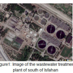
The wastewater treatment plant of south of Isfahan is located in the southeastern part of Isfahan and long the Zayandehrood river and it is located approximately at the 1563 meters above sea level. The first phase of this wastewater treatment plant was begun to work with trickling filter method in the year of 1967 with a capacity of 90000 people. The second and third phases of that were exploited in 1983 and 1987 respectively by the conventional activated sludge method and each of them with a capacity of 400000 people. The influent flow is about 130000 m3/d. The input wastewater after passing the screening and Grit chamber units is entered into the four primary sedimentation tanks that each volume is 2500 cubic meters and with a diameter of 35 meters. Then the wastewater enters into two aerobic thanks at each phase to biological treatment. The total volume of aeration tank is 32400 cubic meters. Then the output wastewaters are entering into 4 secondary sedimentation tanks with a diameter of 60 meter. The volume of each of the secondary sedimentation tank is 8105 cubic meters. The effluent after passing the Chlorine contact tank is navigated to the Zayandehrood river for agricultural uses. In figure 1, the image of wastewater treatment plant of south of Isfahan is visible.
 |
|
Material and Method
The desired samples were obtained from input wastewater, aeration tanks and effluent of wastewater treatment plant of south of Isfahan during 68 days. The values of physical and chemical parameters were examined by the measurement method in the Standard method book (APHA, 2005). TSS, VSS, BOD, sBOD, COD, sCOD were analyzed every day and TN, MLSS, NH4-N, NO3-N were analyzed three timed a week. It is noteworthy that NO3-N and TN parameters were analyzed by using Commercial test kits. To determine MLSS, sBOD, sCOD, the Whatman GF/C glass-fiber filters were used.
Wastewater Characteristic
After doing experiments on the wastewater treatment plant of south of Isfahan, test results were statistically analyzed as summarized in Tables 1 and 2.
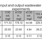 |
Table1: the characteristics of input and output wastewater treatment plant during 68 days experiments Click here to View table |
Table2: the characteristics of wastewater aeration tank during 68-days experiments
|
average |
2982.58 |
2407.46 |
1.65 |
|
standard deviation |
454.74 |
346.60 |
0.21 |
|
C.V |
0.15 |
0.14 |
0.13 |
As can be seen in tables 1 and 2, for the desired parameters in the input, output and inside the aeration tank, mean, standard deviation and coefficient of variation were calculated by using the SPSS software. For example, the average of input and output BOD and COD parameters were obtained 240, 82.5, 575.5, 171.33 mg/l respectively.
In probability theory and statistics, the coefficient of variation (CV) is a normal measure and it is used for measuring the distribution of statistical data. In other words, the coefficient of variation, express the average dispersion for one unit and it is a dimensionless value. this coefficient is a number less than 1 and if it closes to 1, indicates a greater dispersion and if it closes to zero, indicates the lack of proper dispersion and proper correlation of statistical data (Forkman., 2013). According to the statistical results presented in Tables 1 and 2, the range of coefficient of variation for the conducted experiments are between 0.05 to 0.015 and this range indicates the proper correlation between results and their lack of dispersion.
Modeling the Wastewater Treatment of South of Isfahan
For modeling the process in the aeration tank, the ASM1 model was used. In the sedimentation tank, clarifying process and thickening was modeled through dynamic sedimentation tank model. This model was presented by Takacs et al with name of Generic model (Takacs et al., 1991). STOAT 5.0 was used for implementation of model.
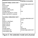
The general plan is entered in the software including primary sedimentation tank, aeration tank and secondary sedimentation tank which is visible in Figure 2. After the above steps, the characteristics of input wastewater, physical dimensions, used model in each unit and some of the operational characteristics were defined for the software and could be seen in figure 3 as a sample. then by running the program, observing the modeling results was possible.
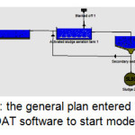 |
Fig. 2: the general plan entered into the STOAT software to start modeling Click here to View figure |
 |
|
Components of ASM1 model: ASM1 model includes 13 components and these values should be determined for the model. Thus according to the experimental results and available information in the wastewater treatment plant of south of Isfahan, below values were determined for some of the components and it was entered to the model which can be seen in Table 3. For other components, the default values for sanitary wastewaters in the software were used.
Table3: the components of ASM1 model for wastewater treatment plant of south of Isfahan
|
parameter |
value |
|
SI .Concentration of inert soluble organic material .mg COD/L |
30.0 |
|
SS .Concentration of readily biodegradable soluble substrate. mg COD/L |
148.12 |
|
XI .Concentration of particulate inert organic matter. mg/L |
161.0 |
|
XS .Concentration of slowly biodegradable particulate substrate. mg COD/L |
235.88 |
|
SO .Concentration of soluble oxygen. mg/L |
1.65 |
|
SND .Concentration of soluble biodegradable organic material. mg N/L |
18.0 |
|
SNH .Concentration of soluble ammonium nitrogen. mg N/L |
43 |
|
SNO .Concentration of soluble nitrate and nitrite nitrogen. mg N/L |
0 |
|
XND .Concentration of particulate biodegradable organic nitrogen. mg COD/L |
4.45 |
According to table 3, the sum of SS, XI, SI and XS parameters will be equal to COD which is equivalent of 575 mg/l. Also the sum of SND، SNH، SNO and XND parameters equal to the total nitrogen concentration minus non-biodegradable nitrogen. The sum of mentioned parameters is equal to 65.45 mg/l. the total input nitrogen according to the experiments is equal to 68.23 mg/l. the amount of difference between them is about 2.78 mg/l and this difference is the non-biodegradable organic nitrogen which is not entered into the ASM1 model. SO is the concentration of dissolved oxygen. According to experiments the average of SO is 1.65 mg/l.
Model Calibration
Model calibration is one of the most important steps of modeling. In this step, the values are assigned to some or all of the kinetic and stoichiometric coefficients and they are based on the conducted experiments on the desired wastewater or they are driven from the results of other researchers. The purpose of the model calibration was to closing the model prediction results and the experiment results. In this study, by using the experimental results and following equations, the values of biokinetic coefficients were calculated (Mardani et al., 2011).
Where SRT is Solids retention time, d and Y is Biomass yield, mg VSS/mg sCOD and U is Substrate utilization rate, mg sCOD/mg VSS.d and kd is Endogenous decay coefficient, 1/d and S0 is Influent substrate concentration, mg sCOD/L and S is Effluent substrate concentration, mg sCOD/L and X is Biomass concentration, mg VSS/L and Ó¨ is Hydraulic retention time, d and Ks is Half-velocity constant, mg sCOD/L and k is Maximum rate of substrate utilization, mg sCOD/mg VSS.d and µm is maximum specific growth rate, 1/d
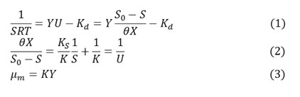
By using the equation 1, the chart of 1/SRT was plotted versus U and by curve fitting; the values of Y and Kd were calculated. On this basis, the Y and Kd coefficients were determined equal to 0.411 VSS/mg sCOD and 0.984 1/d. the chart was shown in figure 4.
 |
|
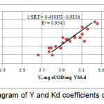
Then, by using equation 2, the chart of 1/U was plotted versus 1/S and by the curve fitting; the amounts of K and Ks were evaluated. In figure 5, the mentioned chart is observable. On this basis, the K and Ks coefficients were determined respectively 20.496 mg sCOD/mg VSS.d and 71.12 mg sCOD/L. in the following, by using the equation 3, the amount of µm coefficient was obtained 8.424 l/d.
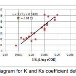 |
Fig. 5: diagram for K and Ks coefficient determination Click here to View figure |
Results and Discussions
To evaluating the results, the results were divided into three groups. The first group includes the effluent carbonaceous compounds, the second group includes the effluent suspended solids and the third group includes the effluent nitrogenous compounds. Then, the closeness rate of experimental results and simulation results were compared.
The effluent total COD includes the biodegradable soluble COD, non-biodegradable soluble COD, particulate biodegradable COD and particulate non-biodegradable COD. The model output is visible in figure 6. Also the obtained results of table 4 are comparable with the model predicted results.
 |
|
Table4: comparison of experimental results with the model prediction results for the carbon compounds
|
parameter |
COD out, mg/l |
sbCOD out , mg/l |
snbCOD out , mg/l |
pbCOD out , mg/l |
pnbCOD out , mg/l |
|
|
experiment |
average |
171.33 |
44.99 |
127.34 |
||
|
model |
average |
167.82 |
48.38 |
119.45 |
||
|
difference |
2.05% |
9.98% |
6.20% |
|||
According to the above table, total predicted COD by the model has a difference about 2% with the conducted experimental results on the effluent of wastewater treatment plant of Isfahan. For each of the COD components, this difference is about 7% and it is an acceptable value. The nonbiodegradable soluble COD in the input of model was considered about 30 mg/l of the inlet COD and as expected, this value remained almost unchanged and at the effluent, it is expected about 29.89 mg/l. the biodegradable soluble COD was applied in the input model about 148.12 mg/l and its amount in the effluent was observed about 14 mg/l and in the output of the model, it was obtained about 18.49 mg/l. According to the experiment results the particulate COD in the effluent was observed about 127.34 mg/l and based on the model output, this amount that is the sum of the biodegradable COD and non-biodegradable COD was predicted about 119.45 mg/l and it has 6% difference with the observed value in the experiments.
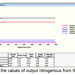
The total output nitrogen includes ammonia nitrogen, organic nitrogen and nitrate nitrogen. The predicted values of the model output can be seen in the figure 7. Also, in table 5, the obtained values of experiments with the predicted results are comparable.
 |
|
Table5: comparison of experimental results with the results of model prediction for the nitrogenous compounds
|
parameter |
TN out, mg/l |
TKN out , mg/l |
NO3-N out, mg/l |
||
|
NH4-N out , mg/l |
Org-N out , mg/l |
||||
|
experiment |
average |
- |
54.47 |
- |
|
|
model |
average |
53.74 |
53.56 |
0.18 |
|
|
difference |
1.67% |
- |
|||
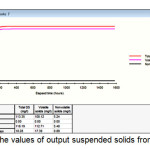
According to Table 5, the observed effluent Kjeldahl nitrogen in the experiments is about 54.47 mg/l which has a very low difference about 1.67% with the predicted value by the model which is equals to 53.56 mg/l. due to the low SRT about 10 days, considerable nitrate is not produced and the difference between input and output nitrogen has been entered to the produced biomass. According to the model results, the produced nitrate was about 0.18 mg/l and dissolved and particulate organic nitrogen were about 8.9 mg/l and the total effluent nitrogen is predicted about 53.74 mg/l. the effluent suspended solids contain volatile suspended solids and non-volatile suspended solids. The output predicted model can be seen in Figure 8. Also, in table 6 the model predicted values and the experimental results are comparable.
 |
|
Table6: comparison of experimental results with the model predicted results for the suspended solids
|
parameter |
TSS out, mg/l |
VSSout, mg/l |
nVSS out, mg/l |
|
|
experiment |
average |
105.33 |
- |
- |
|
model |
average |
113.35 |
108.12 |
5.24 |
|
difference |
7.61% |
- |
||
According to the experimental results, the value of effluent TSS was obtained about 105.33 mg/l and the predicted TSS by the model was about 113.35 mg/l. these two amounts have a difference about 7%. The amounts of VSS and nVSS were predicted by the model, respectively 108.12 and 5.24 mg/l.
Considering the mentioned information, the model output with biokinetic calibrated coefficients is acceptable and the model results with experiments have less than 10% difference. To adopting the model results with the experimental results, we can calibrate other model coefficients by using experiments or manual to obtain the other optimized coefficients.
Conclusions
The wastewater treatment plant of the south of Isfahan was modeled in the STOAT software. For the aeration tank, the ASM1 model and for the secondary sedimentation tank, the Generic model was used. The characteristics of output and input wastewater from the conventional activated sludge of the wastewater treatment plant of the south of Isfahan were measured during 68 days and these were entered into the ASM1 model. To evaluate the results of modeling, the results were divided into three groups. The first group includes the effluent carbonaceous compounds, second group includes the effluent suspended solids and third group includes the effluent nitrogenous compounds. To calibrating the model, the biokinetic coefficients of KS, Kd, K, Y, µm were measured in the 20 centigrade degree and it was used instead of default coefficients. Then the simulation results are compared with the results of the experiments. The experimental results show a good adoption with model outputs and the maximum observed difference is less than 10%.
Acknowledgments
Environment Research Center, Isfahan University of Medical Science (IUMS) Isfahan, Iran; and Department of Environmental Health Engineering, School of Health, student, Research Center, (IUMS), Isfahan, Iran.
References
- American Public Health Association (APHA) Standard Methods for Examination of Water and Wastewater, Washington (2005).
- Barnett, M.W., Takacs, I., Stephenson, J., Gall, B and Perdeus, M., Dynamic modeling. Water Environ Technol, 12, 41–44 (1995).
- Cakici, A and Bayramoglu, M., An approach to controlling sludge age in the activated sludge process. Water Res, 29(4), 1093–1097 (1995).
- Carucci, A., Rolle, E and Smurra, P., Management optimisation of a large wastewater treatment plant. Water Sci Technol, 39(4), 129–136 (1999).
- Fenu, A., Guglielmi, G., Activated sludge model (ASM) based modelling of membrane bioreactor (MBR) processes: A critical review with special regard to MBR speciï¬cities. Water Research, 44, 4274-4294 (2010).
- Forkman, J. Estimator and tests for common coefficients of variation in normal distributions. Communications in Statistics - Theory and Methods , 38, 2013.
- Forkman, J. Estimator and tests for common coefficients of variation in normal distributions. Communications in Statistics - Theory and Methods , 38, 2013.
- IWA Task group on mathematical modelling for design and operation of biological wastewater treatment, Activated sludge models ASM1, ASM2, ASM2D and ASM3. IWA Publishing, London, UK (2000).
- Liwarska-Bizukojc, E and Biernacki, R., Identiï¬cation of the most sensitive parameters in the activated sludge model implemented in BioWin software. Bioresource Technology, 101, 7278–7285 (2010).
- Makinia, J., Swinarski, M and Dobiegala, E., Experiences with computer simulation at two large wastewater treatment plants in northern Poland. Water Sci Technol, 45(6), 209–218 (2002).
- Mardani, Sh., Mirbagheri, A and Amin, M.M., Determination of biokinetic coefficients for activated sludge processes on municipal wastewater. J. Environ. Health. Sci. Eng, ,.4(1), 25–34 (2011).
- Nelson, M.I and Sidhu, H.S., Analysis of the activated sludge model (number 1). Applied Mathematics Letters, 22, 629–635 (2009).
- Nuhoglu, A., Keskinler, B and Yildiz, E., Mathematical modelling of the activated sludge process-the Erzincan case. Process Biochemistry, 40, 2467–2473 (2005).
- Olsson, G and Newell, B., Wastewater treatment systems: modeling diagnosis and control. IWA Publishing, London, UK (1999).
- Ozer, C., Daigger, G.T and Graef, S.P., Evaluation of IAWQ activated sludge model no. 2 using steady-state data from four full-scale wastewater treatment plants. Water Environ Res, 70(6), 1216–1224 (1998).
- Sarkar, U., Dasgupta, D., Bhattacharya, T., Pal, S and Chakroborty, T., Dynamic simulation of activated sludge based wastewater treatment processes: Case studies with Titagarh Sewage Treatment Plant, India. Desalination, 252, 120–126 ( 2010).
- Siegrist, H and Tschui, M.,Interpretation of experimental data with regard to the activated sludge model no. 1 and calibration of the model for municipal wastewater treatment plants. Water Sci Technol, 25(6), 167–831 (1992).
- Takacs, I., Patry, G.G and Nolasco, D. A., dynamic model of the clariï¬cation thickening process. Water Res, 25(10), 1263–1271 (1991).